Step-by-step LC-MS/MS Differential Expression Workflow in R

Proteomics in Biomedicine

Gorka Prieto <gorka.prieto@ehu.eus>

University of the Basque Country (UPV/EHU)

October 5, 2023

Table of contents

• 1 Outline
• 2 Dataset
  • 2.1 iPRG
  • 2.2 MassIVE
  • 2.3 Validation
• 3 Manual workflow
  • 3.1 Importing data
  • 3.2 Label-free quantification
  • 3.3 Normalization
  • 3.4 Imputation
  • 3.5 Differential expression
• 4 More advanced workflows
  • 4.1 MSstats
  • 4.2 Tidyproteomics
  • 4.3 Others
• 5 Exercise
• 6 References
  • 6.1 Tutorials
  • 6.2 Papers

1 Outline

• From quantified peptides/features to differentially expressed proteins (DEPs)
• Using dataset of known composition to validate our results
• Manual steps (more didactic):
  1. Importing quantified peptides
  2. Calculating protein abundance
  3. Normalization and imputation
  4. Calculating fold-changes and p-values
• R packages for more advanced workflows

2 Dataset

2.1 iPRG

Dataset from Choi et al. (2017)

• iPRG 2015 study (bioinformatics part of ABRF)
• 4 samples (1..4) of known composition:
  • 200 ng of tryptic digests of S. cerevisiae
  • Different quantities of 6 individual protein digests
• 3 LC-MS/MS acquisitions (A, B, C) for each sample:
  • Total of 12 runs in random order
• Provided a list of target PSMs

2.2 MassIVE

• MassIVE reanalysis of the iPRG 2015 dataset
• MaxQuant output files (just to avoid raw data search)
• MSstats annotation file

annotation <- read_csv("data/iPRG-2015/quant/MSV000079843_IPRG-annotation_fixed.csv")
annotation %>% arrange(Condition, Experiment)

# A tibble: 12 × 5
   Raw.file              Condition BioReplicate Experiment IsotopeLabelType
   <chr>                 <chr>            <dbl> <chr>      <chr>           
 1 JD_06232014_sample1-A C1                   1 sample1_A  L               
 2 JD_06232014_sample1_B C1                   1 sample1_B  L               
 3 JD_06232014_sample1_C C1                   1 sample1_C  L               
 4 JD_06232014_sample2_A C2                   2 sample2_A  L               
 5 JD_06232014_sample2_B C2                   2 sample2_B  L               
 6 JD_06232014_sample2_C C2                   2 sample2_C  L               
 7 JD_06232014_sample3_A C3                   3 sample3_A  L               
 8 JD_06232014_sample3_B C3                   3 sample3_B  L               
 9 JD_06232014_sample3_C C3                   3 sample3_C  L               
10 JD_06232014_sample4-A C4                   4 sample4_A  L               
11 JD_06232014_sample4_B C4                   4 sample4_B  L               
12 JD_06232014_sample4_C C4                   4 sample4_C  L               

2.3 Validation

spiked <- tibble(
  Protein = c("sp|P44015|VAC2_YEAST", "sp|P55752|ISCB_YEAST", "sp|P44374|SFG2_YEAST", "sp|P44983|UTR6_YEAST",  "sp|P44683|PGA4_YEAST", "sp|P55249|ZRT4_YEAST"),
  spiked = LETTERS[1:6])

spiked

# A tibble: 6 × 2
  Protein              spiked
  <chr>                <chr> 
1 sp|P44015|VAC2_YEAST A     
2 sp|P55752|ISCB_YEAST B     
3 sp|P44374|SFG2_YEAST C     
4 sp|P44983|UTR6_YEAST D     
5 sp|P44683|PGA4_YEAST E     
6 sp|P55249|ZRT4_YEAST F     

3 Manual workflow

3.1 Importing data

• MaxQuant files:

proteinGroups <- read_delim("data/iPRG-2015/quant/proteins.tsv", delim = "\t", escape_double = FALSE, trim_ws = TRUE)
evidence <- read_delim("data/iPRG-2015/quant/evidence.tsv", delim = "\t", escape_double = FALSE, trim_ws = TRUE)

• Combine them using MSstatsConvert

quant <- MaxQtoMSstatsFormat(
  evidence=evidence, annotation=annotation, proteinGroups=proteinGroups,
  useUniquePeptide = TRUE, summaryforMultipleRows = max, removeProtein_with1Peptide=TRUE)

3.1 Importing data

INFO  [2023-10-03 13:14:32] ** Raw data from MaxQuant imported successfully.
INFO  [2023-10-03 13:14:32] ** Rows with values of Potentialcontaminant equal to + are removed 
INFO  [2023-10-03 13:14:32] ** Rows with values of Reverse equal to + are removed 
INFO  [2023-10-03 13:14:33] ** Rows with values of Potentialcontaminant equal to + are removed 
INFO  [2023-10-03 13:14:33] ** Rows with values of Reverse equal to + are removed 
INFO  [2023-10-03 13:14:33] ** Rows with values of Onlyidentifiedbysite equal to + are removed 
INFO  [2023-10-03 13:14:33] ** + Contaminant, + Reverse, + Potential.contaminant, + Only.identified.by.site proteins are removed.
INFO  [2023-10-03 13:14:33] ** Raw data from MaxQuant cleaned successfully.
INFO  [2023-10-03 13:14:33] ** Using provided annotation.
INFO  [2023-10-03 13:14:33] ** Run labels were standardized to remove symbols such as '.' or '%'.
INFO  [2023-10-03 13:14:33] ** The following options are used:
  - Features will be defined by the columns: PeptideSequence, PrecursorCharge
  - Shared peptides will be removed.
  - Proteins with a single feature will be removed.
  - Features with less than 3 measurements across runs will be removed.
INFO  [2023-10-03 13:14:33] ** Features with all missing measurements across runs are removed.
INFO  [2023-10-03 13:14:34] ** Shared peptides are removed.
INFO  [2023-10-03 13:14:34] ** Multiple measurements in a feature and a run are summarized by summaryforMultipleRows: max
INFO  [2023-10-03 13:14:34] ** Features with one or two measurements across runs are removed.
INFO  [2023-10-03 13:14:34] Proteins with a single feature are removed.
INFO  [2023-10-03 13:14:35] ** Run annotation merged with quantification data.
INFO  [2023-10-03 13:14:35] ** Features with one or two measurements across runs are removed.
INFO  [2023-10-03 13:14:35] ** Fractionation handled.
INFO  [2023-10-03 13:14:36] ** Updated quantification data to make balanced design. Missing values are marked by NA
INFO  [2023-10-03 13:14:36] ** Finished preprocessing. The dataset is ready to be processed by the dataProcess function.

3.2 Label-free quantification

• Calculate protein abundance
• Filtering: >2 unique peptides, q-value <= 0.01
• Aggregating MS/MS counts:
  • Adopted from RNA: limma, edgeR, DESeq2
  • Specific for proteomics: DEqMS, PAI, emPAI, APEX
• Using peak intensities:
  • More accurate
  • MSstats, iBAQ, TPA, TOP3, MaxLFQ

• E.g.: sum of peptides intensities (simple)

quant_prot <- quant %>% as_tibble() %>% 
  group_by(ProteinName, Condition, Run) %>% 
  summarise(Abundance = sum(Intensity, na.rm = TRUE)) %>%
  mutate(Abundance = na_if(Abundance, 0)) %>% 
  mutate(Run=str_replace(str_sub(Run,19),"_","-"))
quant_prot %>% head(5) %>% kable()

ProteinName	Condition	Run	Abundance
sp|D6VTK4|STE2_YEAST	C1	1-A	206578000
sp|D6VTK4|STE2_YEAST	C1	1-B	318715000
sp|D6VTK4|STE2_YEAST	C1	1-C	269458000
sp|D6VTK4|STE2_YEAST	C2	2-A	319582000
sp|D6VTK4|STE2_YEAST	C2	2-B	400019000

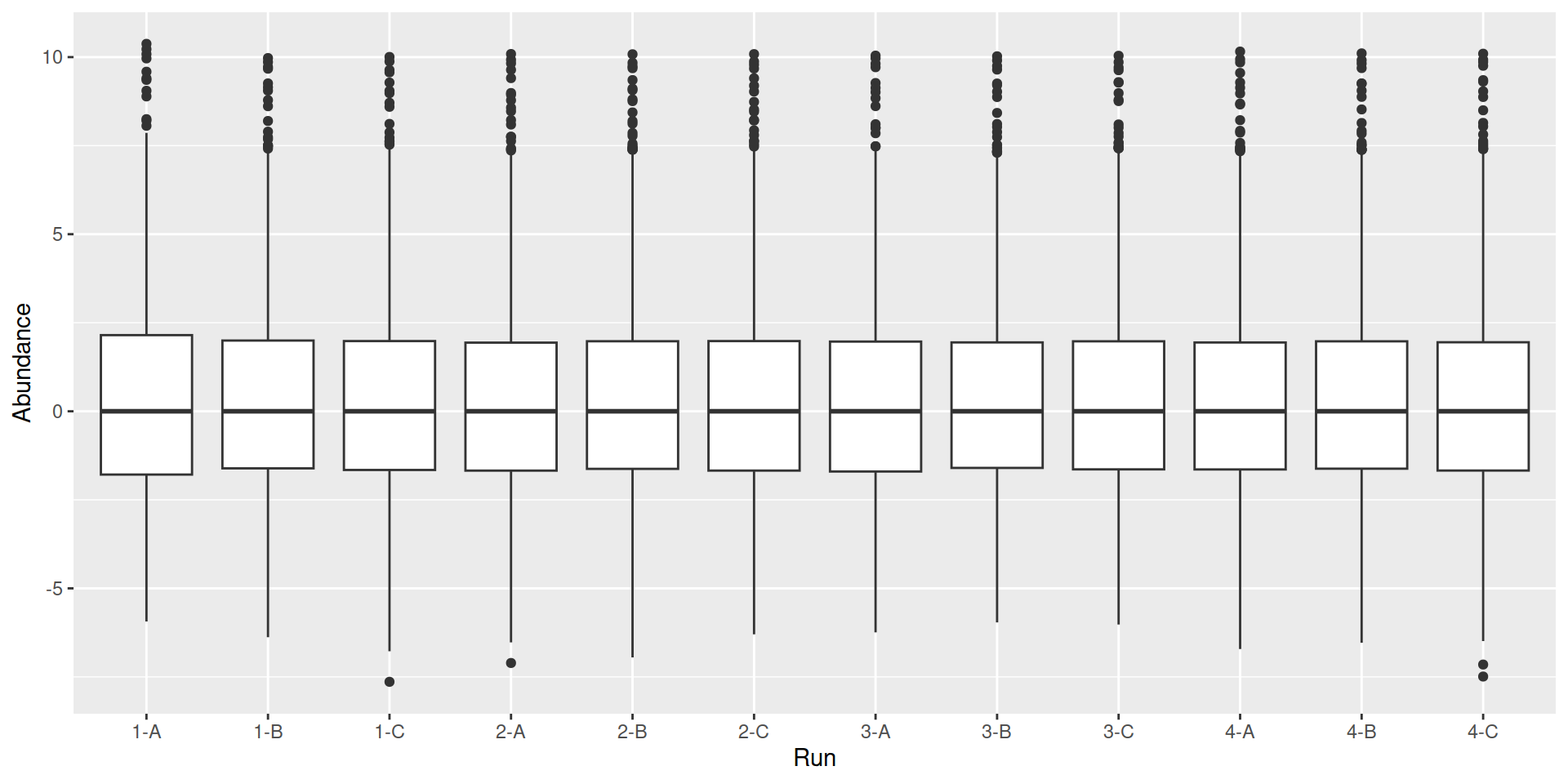
3.3 Normalization

• Account for bias:
  • Make the samples more comparable
  • Analysis more reliable
• Steps:
  • log2 scale (more convenient)
  • Center on the median (next section for more advanced)

quant_norm <- quant_prot %>% 
  mutate(Abundance=log2(Abundance)) %>% 
  group_by(Run) %>% 
  mutate(Abundance=Abundance-median(Abundance, na.rm=TRUE)) %>% 
  ungroup()

quant_norm %>% 
  ggplot(aes(x=Run, y=Abundance)) +
  geom_boxplot()

3.3 Normalization

3.4 Imputation

Missing values

• High rate of missing values in label-free quantitative proteomics
• E.g. % of proteins with at least one NA in any condition:

quant_norm %>% group_by(ProteinName) %>%
  summarise(missing = any(is.na(Abundance))) %>%
  pull(missing) %>% mean() * 100

[1] 8.427362

• Missing [Completely] At Random (MCAR/MAR):
  • Result of stochastic nature of LC-MS/MS
• Missing Not At Random (MNAR):
  • Absence, low abundance, limit of detection (left-censored)

Imputation strategies

• Drop NA is perfect if %missing negligible
• Replace missing values: zero, minimum, Gaussian (minimum), kNN, etc.
• Lazar et al. (2016):
  • Best imputation strategies depend on MAR/MNAR nature
  • Peptide-level vs protein-level imputation
  • Hybrid strategies are ideal, MAR if in doubt
• E.g. use minimum value in each run (simple):

quant_imp <- quant_norm %>% 
  group_by(Run) %>% 
  mutate(Abundance=ifelse(is.na(Abundance), min(Abundance, na.rm = TRUE), Abundance)) %>% 
  ungroup()

3.5 Differential expression

• Log2 fold-change of protein mean abundance between conditions
• Student’s t-test to calculate p-values
• Benjamini-Hochberg (BH) to adjust p-values
• E.g. C4 vs C1:

quant_dep <- quant_imp %>% 
  filter(Condition == "C1" | Condition == "C4") %>% 
  group_by(ProteinName, Condition) %>% 
  mutate(mean = mean(Abundance)) %>% 
  ungroup() %>% 
  pivot_wider(names_from = Condition, values_from = mean) %>% 
  pivot_wider(names_from = Run, values_from = Abundance) %>% 
  group_by(ProteinName) %>% 
  summarise(across(everything(), ~first(na.omit(.x)))) %>% 
  mutate(Log2FC = C4-C1) %>% 
  rowwise() %>% 
  mutate(pval = t.test(c(`1-A`, `1-B`, `1-C`), c(`4-A`, `4-B`, `4-C`), alternative = "two.sided", var.equal = TRUE)$p.value) %>% 
  ungroup() %>% 
  mutate(padj = p.adjust(pval, method = "BH")) %>% 
  merge(spiked %>% rename(ProteinName=Protein), all.x = TRUE)

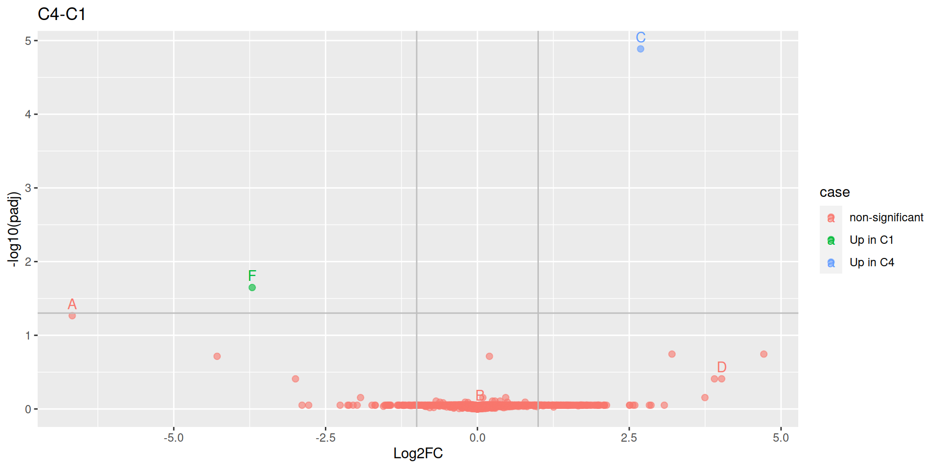
Results

quant_dep <- quant_dep %>%
  mutate(case = ifelse(abs(Log2FC)<1 | padj>0.05, "non-significant", NA)) %>% 
  mutate(case = ifelse(is.na(case) & Log2FC <= -1, "Up in C1", case)) %>% 
  mutate(case = ifelse(is.na(case) & Log2FC >= 1, "Up in C4", case))

quant_dep %>%
  filter(!is.na(spiked)) %>%
  select(spiked, Log2FC, pval, padj, case) %>% 
  arrange(spiked) %>% kable()

spiked	Log2FC	pval	padj	case
A	-6.6722882	0.0000573	0.0542040	non-significant
B	0.0487597	0.7523559	0.9411774	non-significant
C	2.6870814	0.0000000	0.0000130	Up in C4
D	4.0214733	0.0010991	0.3896386	non-significant
F	-3.7089754	0.0000159	0.0224813	Up in C1

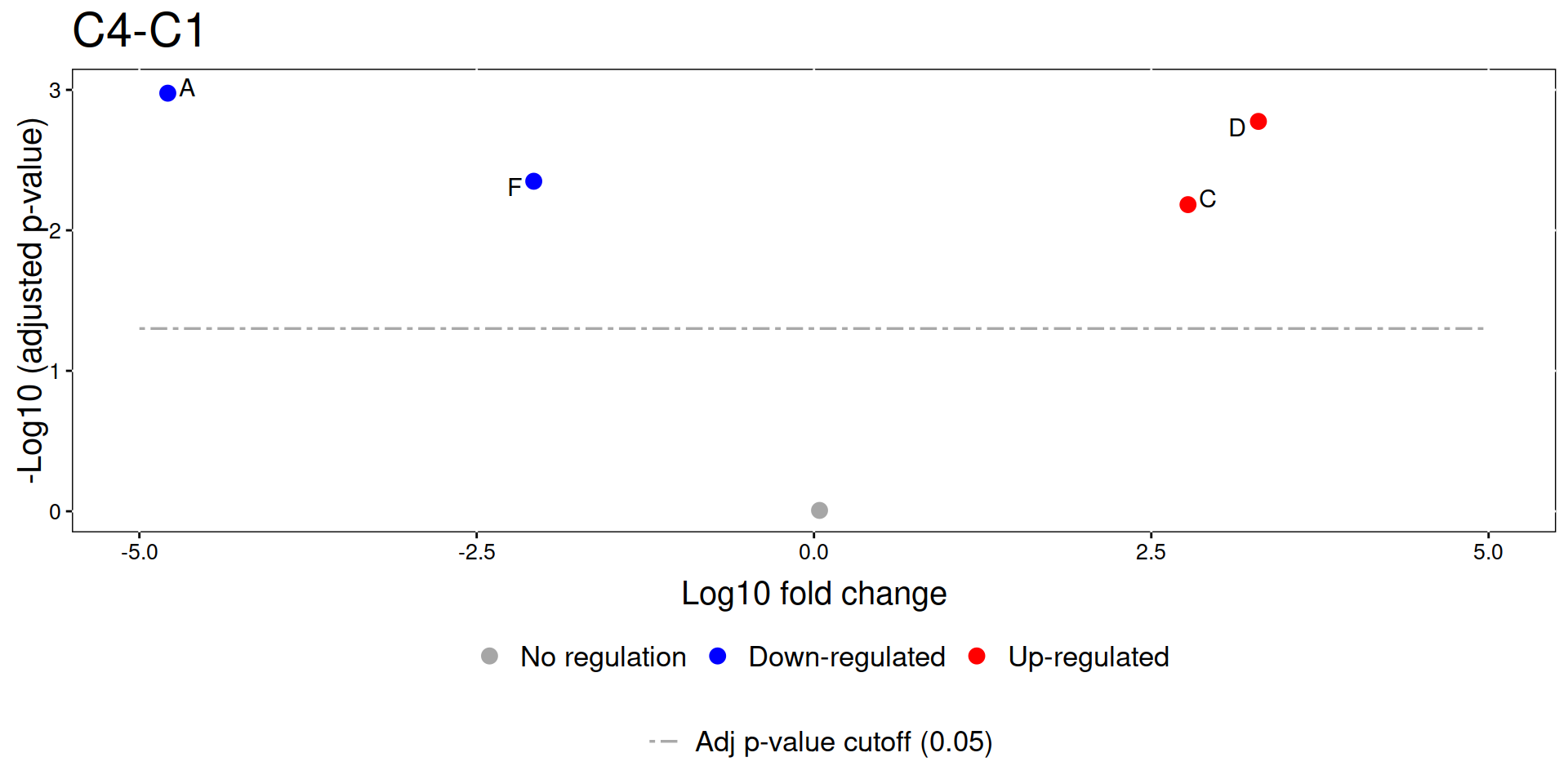
Volcano plot

quant_dep %>%
  ggplot(aes(x=Log2FC, y=-log10(padj), color=case)) +
  geom_point(shape=19, size=2, alpha = 0.6) +
  geom_vline(xintercept = c(-1, 1), color = "grey") +
  geom_hline(yintercept = -log10(0.05), color = "grey") +
  geom_text(aes(label=spiked), hjust = 0.5, vjust = -0.6) +
  ggtitle("C4-C1")

Volcano plot

4 More advanced workflows

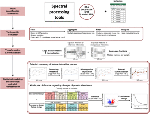
4.1 MSstats

• See Kohler et al. (2023)

Processing data

• dataProcess():
  • Transformation to log scale
  • Different normalization options
  • Different feature aggregation options
  • Imputation

quant_processed <- dataProcess(quant,
  logTrans = 2,
  normalization = "equalizeMedians",
  summaryMethod="TMP",
  censoredInt="NA",
  MBimpute=TRUE,
  featureSubset="all",
  min_feature_count = 2,
  n_top_feature=3,
  remove_uninformative_feature_outlier=TRUE,
  maxQuantileforCensored=0.999)

Comparison

comparison <- tibble(comparison="C4-C1", C1=-1, C2=0, C3=0, C4=1) %>%
  column_to_rownames("comparison") %>% as.matrix()

quant_comp <- groupComparison(contrast.matrix=comparison, data=quant_processed)
quant_comp <- quant_comp$ComparisonResult

quant_comp %>% 
  merge(spiked) %>% 
  mutate(Protein=spiked) %>% 
  arrange(Protein) %>% 
  select(Protein, log2FC, pvalue, adj.pvalue) %>% 
  kable()

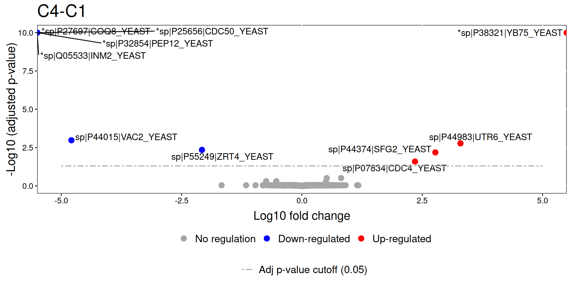
Protein	log2FC	pvalue	adj.pvalue
A	-4.7895044	0.0000004	0.0010560
B	0.0411127	0.9002167	0.9856256
C	2.7720778	0.0000093	0.0065627
D	3.2939558	0.0000012	0.0016771
F	-2.0770543	0.0000047	0.0044728

Visualization

groupComparisonPlots(data=quant_comp, type="VolcanoPlot", address=FALSE)

quant_comp %>% merge(spiked) %>% mutate(Protein=spiked) %>%
  groupComparisonPlots(type="VolcanoPlot",address=FALSE) +
  geom_text(aes(label=spiked))

NULL

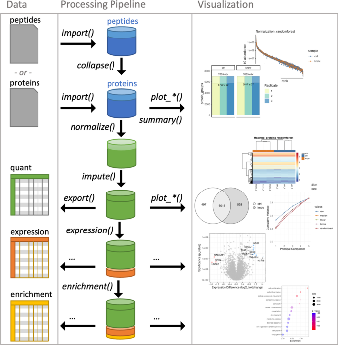
4.2 Tidyproteomics

• See Jones et al. (2023)

Steps

1. Importing:

tp_peptides <- tidyproteomics::import("data/iPRG-2015/quant/evidence.tsv", "MaxQuant", "peptides")

2. Collapsing into proteins:

tp_proteins <- tp_peptides %>% 
  tidyproteomics::collapse(assign_by = 'non-homologous', top_n = Inf, .function = fsum)

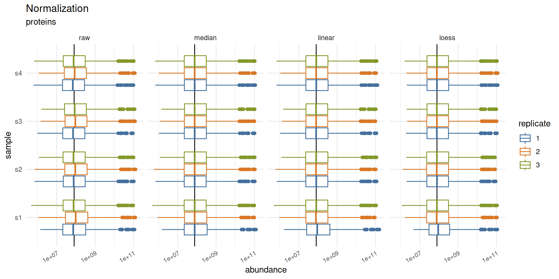
3. Normalization:

tp_norm <- tp_proteins %>%
  tidyproteomics::normalize(.method = c('median', 'linear', 'loess'))

tidyproteomics::plot_normalization(tp_norm)

Steps

4. Imputation:

tp_imp <- tp_norm %>% 
  tidyproteomics::impute(.function = impute.randomforest, method = 'matrix')

5. Differential expression:

tp_dep <- tp_imp %>% 
  tidyproteomics::expression(s4/s1)

tp_dep$analysis$`s4/s1` %>%
  merge(spiked %>% mutate(expression.protein=str_split_i(Protein, "\\|", 2))) %>%
  select(spiked, expression.log2_foldchange, expression.p_value, expression.adj_p_value) %>% 
  arrange(spiked)

  spiked expression.log2_foldchange expression.p_value expression.adj_p_value
1      A               -6.321226216       1.142007e-03             0.92502540
2      B                0.009215171       5.119089e-01             0.93139037
3      C                2.722546710       1.647832e-05             0.05056278
4      D                3.563682003       6.044304e-05             0.06527848
5      F               -3.630661529       3.121160e-05             0.05056278

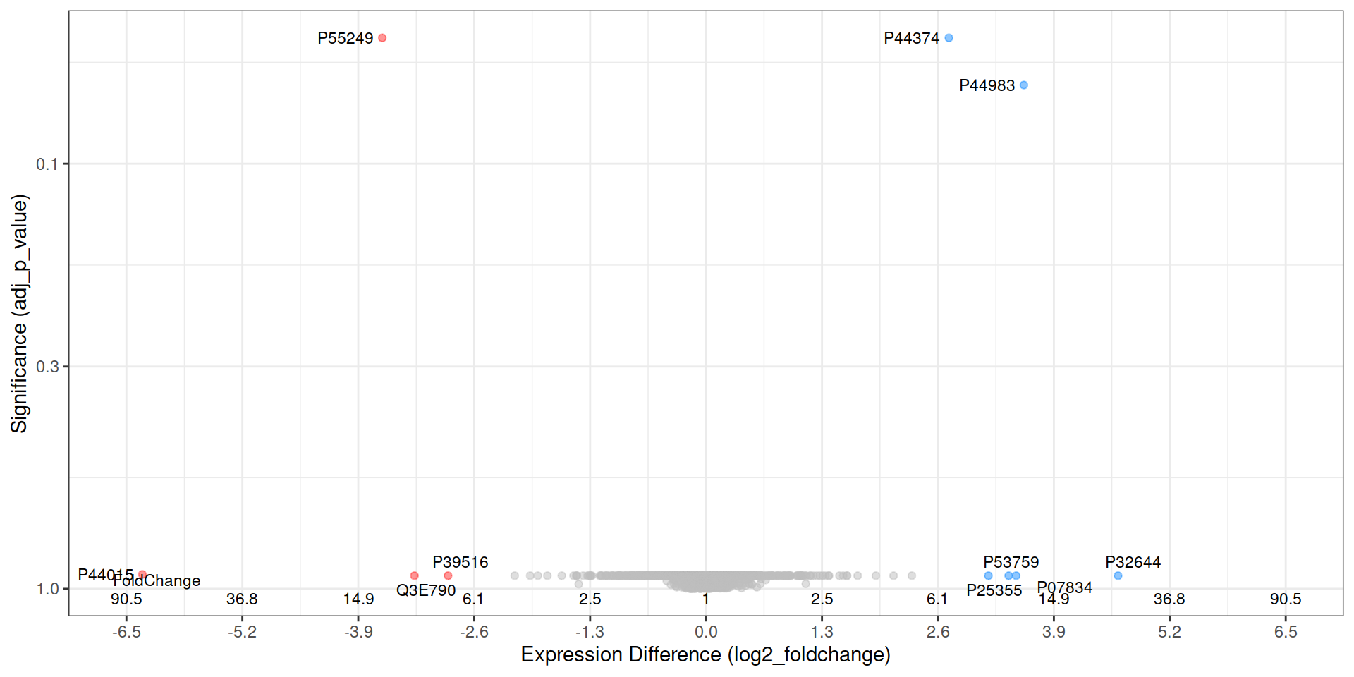
tidyproteomics::plot_volcano(tp_dep, s4/s1)

tp_dep

Origin          MaxQuant 
                proteins (5.49 MB) 
Composition     12 files 
                4 samples (s4, s3, s2, s1) 
Quantitation    3240 proteins 
                4 log10 dynamic range 
                5.25% missing values 
 *normalized    loess 
 *imputed       'matrix' samples via 'impute.randomforest' group_by_sample 'FALSE'. 
Accounting      (3) num_peptides num_unique_peptides imputed 
Analyses        (1) 
                s4/s1 -> expression  
                 

4.3 Others

• Rscript S1 from Choi et al. (2017)
• DDA_iPRG2015_MaxQuant_1.6.script.r from MassIVE reanalysis

5 Exercise

1. Compare the expression levels of the spiked in proteins between two other samples of the provided dataset

6 References

6.1 Tutorials

• Embrace R to Boost Your Proteomic Analysis
• MSstats and MSstatsConvert
• Tidyproteomics
• MSnbase
• R/Bioconductor tools for mass spectrometry-based proteomics
• DEqMS
• DEP
• msqrob2
• Quantitative features for mass spectrometry data
• DAPAR and ProStaR
• OpenMS

6.2 Papers

Choi, Meena, Zeynep F. Eren-Dogu, Christopher Colangelo, John Cottrell, Michael R. Hoopmann, Eugene A. Kapp, Sangtae Kim, et al. 2017. “ABRF Proteome Informatics Research Group (iPRG) 2015 Study: Detection of Differentially Abundant Proteins in Label-Free Quantitative LC–MS/MS Experiments.” Journal of Proteome Research 16 (2): 945–57. https://doi.org/10.1021/acs.jproteome.6b00881.

Jones, Jeff, Elliot J. MacKrell, Ting-Yu Wang, Brett Lomenick, Michael L. Roukes, and Tsui-Fen Chou. 2023. “Tidyproteomics: An Open-Source r Package and Data Object for Quantitative Proteomics Post Analysis and Visualization.” BMC Bioinformatics 24 (1): 239. https://doi.org/10.1186/s12859-023-05360-7.

Kohler, Devon, Mateusz Staniak, Tsung-Heng Tsai, Ting Huang, Nicholas Shulman, Oliver M. Bernhardt, Brendan X. MacLean, et al. 2023. “MSstats Version 4.0: Statistical Analyses of Quantitative Mass Spectrometry-Based Proteomic Experiments with Chromatography-Based Quantification at Scale.” Journal of Proteome Research 22 (5): 1466–82. https://doi.org/10.1021/acs.jproteome.2c00834.

Lazar, Cosmin, Laurent Gatto, Myriam Ferro, Christophe Bruley, and Thomas Burger. 2016. “Accounting for the Multiple Natures of Missing Values in Label-Free Quantitative Proteomics Data Sets to Compare Imputation Strategies.” Journal of Proteome Research 15 (4): 1116–25. https://doi.org/10.1021/acs.jproteome.5b00981.